6.3 Enzyme Kinetics as an Approach to Understanding Mechanism
Biochemists commonly use several approaches to study the mechanism of action of purified enzymes. The three-dimensional structure of the protein provides important information, which is enhanced by traditional protein chemistry and modern methods of site-directed mutagenesis (changing the amino acid sequence of a protein by genetic engineering; see Fig. 9-10). These technologies permit enzymologists to examine the role of individual amino acids in enzyme structure and action. However, the oldest approach to understanding enzyme mechanisms, and one that remains very important, is to determine the rate of a reaction and how it changes in response to changes in experimental parameters, a discipline known as enzyme kinetics. We provide here a basic introduction to the kinetics of enzyme-catalyzed reactions.
Substrate Concentration Affects the Rate of Enzyme-Catalyzed Reactions
At any given instant in an enzyme-catalyzed reaction, the enzyme exists in two forms: the free or uncombined form E and the substrate-combined form ES. When the enzyme is first mixed with a large excess of substrate, there is an initial transient period, the pre–steady state, during which the concentration of ES builds up. For most enzymatic reactions, this period is very brief. The pre-steady state is frequently too short to be observed easily, lasting only the time (often microseconds) required to convert one molecule of substrate to product (one enzymatic turnover). The reaction quickly achieves a steady state in which [ES] (and the concentrations of any other intermediates) remains approximately constant for much of the remainder of the reaction (Fig. 6-10). As most of the reaction reflects the steady state, the traditional analysis of reaction rates is referred to as steady-state kinetics.
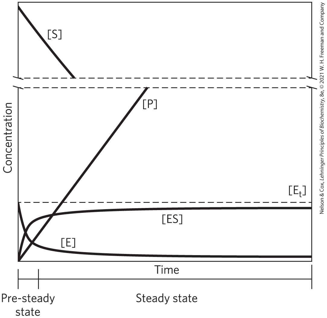
FIGURE 6-10 The course of an enzyme-catalyzed reaction. In a typical reaction, product will increase as substrate declines. The concentration of free enzyme, E, declines rapidly, as the concentration of the ES complex increases and reaches a steady state. The steady-state concentration of ES remains nearly constant for much of the remainder of the reaction.
A key factor affecting the rate of a reaction catalyzed by an enzyme is the concentration of substrate, [S]. However, studying the effects of substrate concentration is complicated by the fact that [S] changes during the course of an in vitro reaction as substrate is converted to product. One simplifying approach is to measure the initial rate (or initial velocity), designated (Fig. 6-11). In a typical reaction, the enzyme may be present in nanomolar quantities, whereas [S] may be five or six orders of magnitude higher. If only the beginning of the reaction is monitored, over a period in which only a small percentage of the available substrate (<2%−3%) is converted to product, [S] can be regarded as constant, to a reasonable approximation. can then be explored as a function of [S], which is adjusted by the investigator. Note that even the initial rate reflects a steady state.
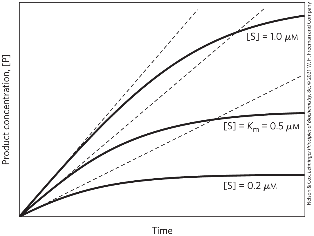
FIGURE 6-11 Initial velocities of enzyme-catalyzed reactions. A theoretical enzyme that catalyzes the reaction is present at a concentration of S sufficient to catalyze the reaction at a maximum velocity, defined as , of 1 μm/min. The rate observed at a given concentration of S depends on the Michaelis constant, , explained in more detail in the next section. Here, the is 0.5 μm. Progress curves are shown for substrate concentrations below, at, and above the . The rate of an enzyme-catalyzed reaction declines as substrate is converted to product. A tangent to each curve taken at time = 0 (dashed line) defines the initial velocity, , of each reaction.
The effect on of varying [S] when the enzyme concentration is held constant is shown in Figure 6-12. At relatively low concentrations of substrate, increases almost linearly with an increase in [S]. At higher substrate concentrations, increases by smaller and smaller amounts in response to increases in [S]. Finally, a point is reached beyond which increases in are vanishingly small as [S] increases. This plateau-like region is close to the maximum velocity, .
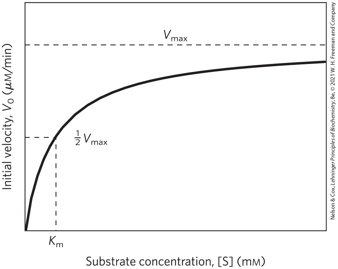
FIGURE 6-12 Effect of substrate concentration on the initial velocity of an enzyme-catalyzed reaction. The maximum velocity, , is extrapolated from the plot, because approaches but never quite reaches . The substrate concentration at which is half-maximal is , the Michaelis constant. The concentration of enzyme in an experiment such as this is generally so low that [S]≫[E] even when [S] is described as low or relatively low. The units shown are typical for enzyme-catalyzed reactions and are given only to help illustrate the meaning of and [S]. (Note that the curve describes part of a rectangular hyperbola, with one asymptote at . If the curve were continued below [S] = 0, it would approach a vertical asymptote at .)
The ES complex is the key to understanding this kinetic behavior, just as it was a starting point for our discussion of catalysis. The kinetic pattern in Figure 6-12 led Victor Henri, following a proposal by Adolphe Wurtz a few decades earlier, to propose in 1903 that the combination of an enzyme with its substrate molecule to form an ES complex is a necessary step in enzymatic catalysis. This idea was expanded into a general theory of enzyme action, particularly by Leonor Michaelis and Maud Menten in 1913. They postulated that the enzyme first combines reversibly with its substrate to form an enzyme-substrate complex in a relatively fast reversible step:
(6-7)
The ES complex then breaks down in a slower second step to yield the free enzyme and the reaction product P:
(6-8)
Because the slower second reaction (Eqn 6-8) must limit the rate of the overall reaction, the overall rate must be proportional to the concentration of the species that reacts in the second step — that is, ES.
Left: Leonor Michaelis, 1875–1949; Right: Maud Menten, 1879–1960
At low [S], most of the enzyme is in the uncombined form E. Here, the rate is proportional to [S] because the equilibrium of Equation 6-7 is pushed toward formation of more ES as [S] increases. The maximum initial rate of the catalyzed reaction is observed when virtually all the enzyme is present as the ES complex and [E] is vanishingly small. Under these conditions, the enzyme is “saturated” with its substrate, so that further increases in [S] have no effect on rate. This condition exists when [S] is sufficiently high that essentially all the free enzyme has been converted to the ES form. After the ES complex breaks down to yield the product P, the enzyme is free to catalyze the reaction of another molecule of substrate (and will do so rapidly under saturating conditions). The saturation effect is a distinguishing characteristic of enzymatic catalysts and is responsible for the plateau observed in Figure 6-12, and the pattern seen in the figure is sometimes referred to as saturation kinetics.
The Relationship between Substrate Concentration and Reaction Rate Can Be Expressed with the Michaelis-Menten Equation
The curve expressing the relationship between [S] and (Fig. 6-12) has the same general shape for most enzymes (it approaches a rectangular hyperbola), which can be expressed algebraically by the Michaelis-Menten equation. Michaelis and Menten derived this equation starting from their basic hypothesis that the rate-limiting step in enzymatic reactions is the breakdown of the ES complex to product and free enzyme. The equation is
(6-9)
This is the Michaelis-Menten equation, the rate equation for a one-substrate enzyme-catalyzed reaction. It is a statement of the quantitative relationship between the initial velocity , the maximum velocity , and the initial substrate concentration [S], all related through a constant, , called the Michaelis constant. All these terms — [S], , , and — are readily measured experimentally.
Here we develop the basic logic and the algebraic steps in a modern derivation of the Michaelis-Menten equation, which includes the steady-state assumption, a concept introduced by G. E. Briggs and J. B. S. Haldane in 1925. The derivation starts with the two basic steps of the formation and breakdown of ES (Eqns 6-7 and 6-8). Early in the reaction, the concentration of the product, [P], is negligible, and we make the simplifying assumption that the reverse reaction, (described by ), can be ignored. This assumption is not critical but it simplifies our task. The overall reaction then reduces to
(6-10)
is determined by the breakdown of ES to form product, which is determined by [ES]:
(6-11)
Because [ES] in Equation 6-11 is not easily measured experimentally, we must begin by finding an alternative expression for this term. First, we introduce the term , representing the total enzyme concentration (the sum of free and substrate-bound enzyme). Free or unbound enzyme [E] can then be represented by . Also, because [S] is ordinarily far greater than , the amount of substrate bound by the enzyme at any given time is negligible compared with the total [S]. With these conditions in mind, the following steps lead us to an expression for in terms of easily measurable parameters.
Step 1 The rates of formation and breakdown of ES are determined by the steps governed by the rate constants (formation) and (breakdown to reactants and products, respectively), according to the expressions
(6-12)
(6-13)
Step 2 We now make an important assumption: that the initial rate of reaction reflects a steady state in which [ES] is constant — that is, the rate of formation of ES is equal to the rate of its breakdown. This is called the steady-state assumption. The expressions in Equations 6-12 and 6-13 can be equated for the steady state, giving
(6-14)
Step 3 In a series of algebraic steps, we now solve Equation 6-14 for [ES]. First, the left side is multiplied out and the right side simplified to give
(6-15)
Adding the term to both sides of the equation and simplifying gives
(6-16)
We then solve this equation for [ES]:
(6-17)
This can now be simplified further, combining the rate constants into one expression:
(6-18)
The term is defined as the Michaelis constant, . Substituting this into Equation 6-18 simplifies the expression to
(6-19)
Step 4 We can now express in terms of [ES]. Substituting the right side of Equation 6-19 for [ES] in Equation 6-11 gives
(6-20)
This equation can be simplified further. Because the maximum velocity occurs when the enzyme is saturated (that is, when ), can be defined as . Substituting this in Equation 6-20 gives Equation 6-9:
Note that has units of molar concentration. Does the equation fit experimental observations? Yes; we can confirm this by considering the limiting situations where [S] is very low or very high, as shown in Figure 6-13.
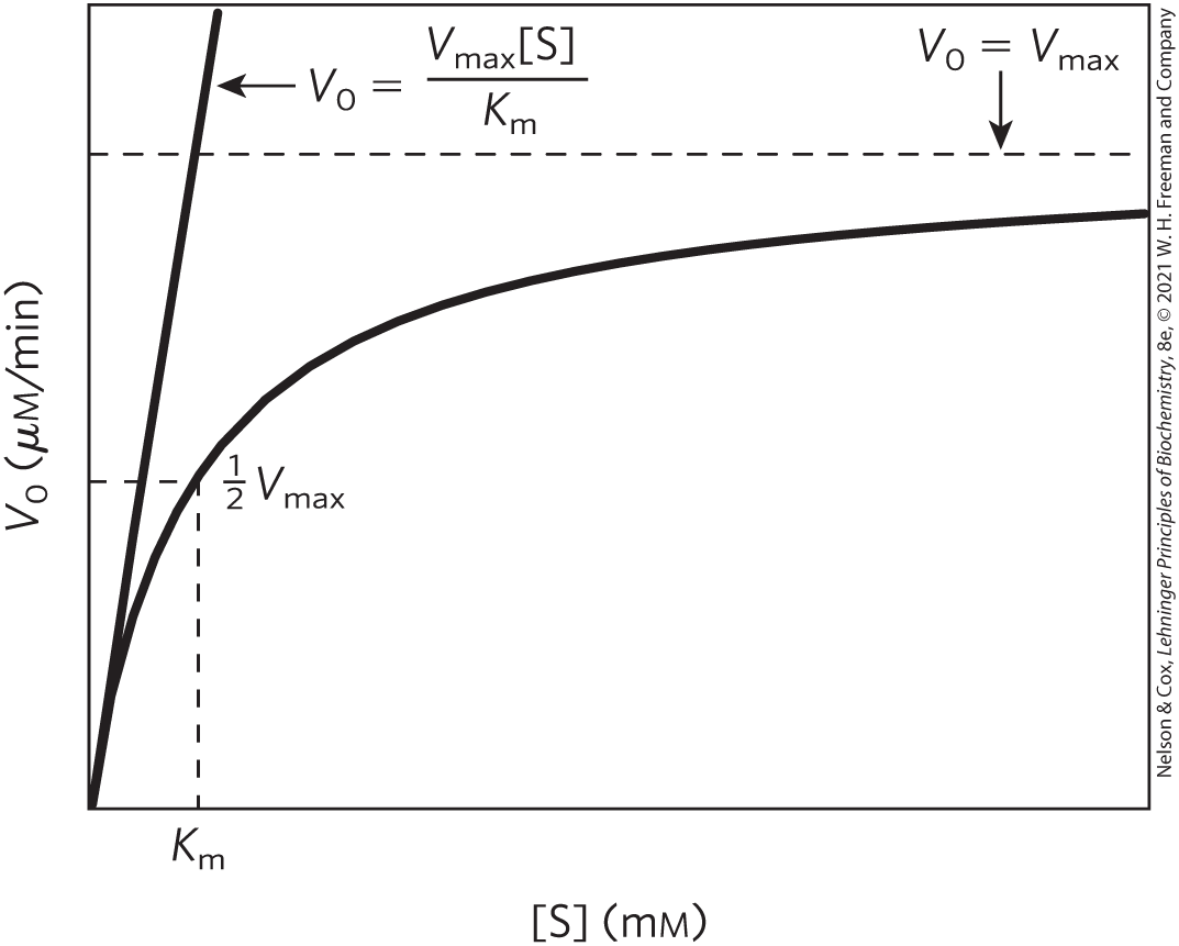
FIGURE 6-13 Dependence of initial velocity on substrate concentration. This graph shows the kinetic parameters that define the limits of the curve at low [S] and high [S]. At low [S], , and the [S] term in the denominator of the Michaelis-Menten equation (Eqn 6-9) becomes insignificant. The equation simplifies to , and exhibits a linear dependence on [S], as observed here. At high [S], where , the term in the denominator of the Michaelis-Menten equation becomes insignificant and the equation simplifies to ; this is consistent with the plateau observed at high [S]. The Michaelis-Menten equation is therefore consistent with the observed dependence of on [S], and the shape of the curve is defined by the terms at low [S] and at high [S].
An important numerical relationship emerges from the Michaelis-Menten equation in the special case when is exactly one-half (Fig. 6-13). Then
(6-21)
On dividing by , we obtain
(6-22)
Solving for , we get , or
when
(6-23)
This is a very useful, practical definition of is equivalent to the substrate concentration at which is one-half .
Michaelis-Menten Kinetics Can Be Analyzed Quantitatively
There are several ways to determine and from a plot relating to [S]. A traditional approach is to algebraically transform the Michaelis-Menten equation into equations that convert the hyperbolic curve in the versus [S] plot into a linear form from which values of and may be obtained by extrapolation. The most common of these approaches takes the reciprocal of both sides of the Michaelis-Menten equation (Eqn 6-9):
(6-24)
Separating the components of the numerator on the right side of the equation gives
(6-25)
which simplifies to
(6-26)
This form of the Michaelis-Menten equation is called the Lineweaver-Burk equation. For enzymes obeying the Michaelis-Menten relationship, a plot of versus 1/[S] (the “double reciprocal” of the versus [S] plot we have been using up to this point) yields a straight line (Fig. 6-14). This line has a slope of , an intercept of on the axis, and an intercept of on the 1/[S] axis. The Lineweaver-Burk plot is a useful way to display data and can provide some mechanistic information, as we will see. However, the double-reciprocal transformation tends to give undue weight to data obtained at low substrate concentration, and can distort errors in the extrapolated values of and .
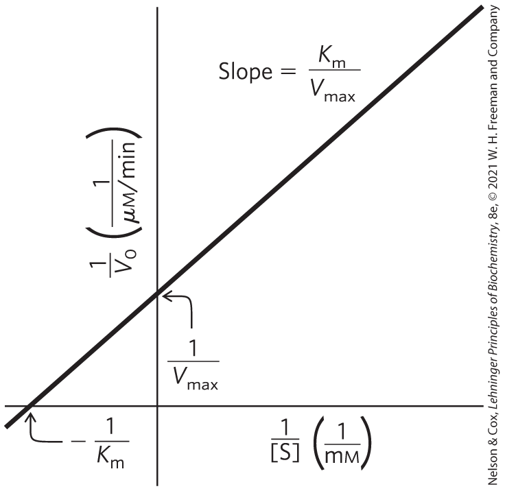
FIGURE 6-14 A double-reciprocal, or Lineweaver-Burk, plot. Plotting versus 1/[S] puts the data into a linear form. Intercepts on the and 1/[S] axes are and , respectively.
More commonly, the parameters and are derived directly from the versus [S] plot via nonlinear regression, using one of a multitude of curve-fitting programs available online. These are generally easy to use and offer accuracy superior to Lineweaver-Burk or related approaches.
Kinetic Parameters Are Used to Compare Enzyme Activities
It is important to distinguish between the Michaelis-Menten equation and the specific kinetic mechanism on which the equation was originally based. The Michaelis-Menten equation does not depend on the relatively simple two-step reaction mechanism proposed by Michaelis and Menten (Eqn 6-10). All enzymes that exhibit a hyperbolic dependence of on [S] are said to follow Michaelis-Menten kinetics. Many enzymes that follow Michaelis-Menten kinetics have quite different reaction mechanisms, and enzymes that catalyze reactions with six or eight identifiable steps often exhibit the same steady-state kinetic behavior. The practical rule that when (Eqn 6-23) holds for all enzymes that follow Michaelis-Menten kinetics. The most important exceptions to Michaelis-Menten kinetics are the regulatory enzymes, discussed in Section 6.5.
The parameters and can be obtained experimentally for any given enzyme, and their measurement is often a key first step in enzyme characterization. However, the mechanistic insight they offer is limited. Obtaining information about the number, rates, or chemical nature of discrete steps in the reaction usually requires additional complementary approaches. Steady-state kinetics nevertheless is the standard language through which biochemists compare and characterize the catalytic efficiencies of enzymes.
Interpreting and
Both the magnitude and the meaning of and can vary greatly from enzyme to enzyme.
can vary even for different substrates of the same enzyme (Table 6-6). The term is sometimes used (often inappropriately) as an indicator of the affinity of an enzyme for its substrate. The actual meaning of depends on specific aspects of the reaction mechanism, such as the number and relative rates of the individual steps. For reactions with two steps,
(6-27)
| Enzyme | Substrate | |
|---|---|---|
| Hexokinase (brain) |
|
|
| Carbonic anhydrase | 26 | |
| Chymotrypsin |
|
|
| β-Galactosidase | d-Lactose | 4.0 |
| Threonine dehydratase | l-Threonine | 5.0 |
When is rate-limiting, , and reduces to , which is defined as the dissociation constant, , of the ES complex. Where these conditions hold, does represent a measure of the affinity of the enzyme for its substrate in the ES complex. However, this scenario does not apply for most enzymes. Sometimes , and then . In other cases, and are comparable, and remains a more complex function of all three rate constants (Eqn 6-27). The Michaelis-Menten equation and the characteristic saturation behavior of the enzyme still apply, but cannot be considered a simple measure of substrate affinity. Even more common are cases in which the reaction goes through several steps after formation of ES; can then become a very complex function of many rate constants.
The quantity depends upon the rate-limiting step of the enzyme-catalyzed reaction. If an enzyme reacts by the two-step Michaelis-Menten mechanism, , where is rate-limiting. However, the number of reaction steps and the identity of the rate-limiting step(s) can vary from enzyme to enzyme. For example, consider the common situation where product release, , is rate-limiting. Early in the reaction (when [P] is low), the overall reaction can be adequately described by the scheme
(6-28)
In this case, most of the enzyme is in the EP form at saturation, and .
It is useful to define a more general rate constant, , to describe the limiting rate of any enzyme-catalyzed reaction at saturation. If the reaction has several steps, one of which is clearly rate-limiting, is equivalent to the rate constant for that limiting step. For the simple reaction of Equation 6-10, . For the reaction of Equation 6-28, when product release is clearly rate-limiting, . When several steps are partially rate-limiting, can become a complex function of several of the rate constants that define each individual reaction step. In the Michaelis-Menten equation, . Rearranged, and Equation 6-9 becomes
(6-29)
The constant is a first-order rate constant and hence has units of reciprocal time. It is also called the turnover number. It is equivalent to the number of substrate molecules converted to product in a given unit of time on a single enzyme molecule when the enzyme is saturated with substrate. The turnover numbers of several enzymes are given in Table 6-7.
| Enzyme | Substrate | |
|---|---|---|
| Catalase | 40,000,000 | |
| Carbonic anhydrase | 400,000 | |
| Acetylcholinesterase | Acetylcholine | 14,000 |
| β-Lactamase | Benzylpenicillin | 2,000 |
| Fumarase | Fumarate | 800 |
| RecA protein (an ATPase) | ATP | 0.5 |
Comparing Catalytic Mechanisms and Efficiencies
The kinetic parameters and are useful for the study and comparison of different enzymes, whether their reaction mechanisms are simple or complex. Each enzyme has values of and that reflect the cellular environment, the concentration of substrate normally encountered in vivo by the enzyme, and the chemistry of the reaction being catalyzed.
The parameters and also allow us to evaluate the kinetic efficiency of enzymes, but either parameter alone is insufficient for this task. Two enzymes catalyzing different reactions may have the same (turnover number), yet the rates of the uncatalyzed reactions may be different and thus the rate enhancements brought about by the enzymes may differ greatly. Experimentally, the for an enzyme tends to be similar to the cellular concentration of its substrate. An enzyme that acts on a substrate present at a very low concentration in the cell usually has a lower than an enzyme that acts on a substrate that is more abundant.
The best way to compare the catalytic efficiencies of different enzymes or the turnover of different substrates by the same enzyme is to compare the ratio for the two reactions. This parameter, sometimes called the specificity constant, is the rate constant for the conversion of E + S to E + P. When , Equation 6-29 reduces to the form
(6-30)
in this case depends on the concentration of two reactants, and [S], so this is a second-order rate equation, and the constant is a second-order rate constant with units of . There is an upper limit to , imposed by the rate at which E and S can diffuse together in an aqueous solution. This diffusion-controlled limit is to , and many enzymes have a near this range (Table 6-8). Such enzymes are said to have achieved catalytic perfection. Note that different values of and can produce the maximum ratio.
| Enzyme | Substrate | |||
|---|---|---|---|---|
| Acetylcholinesterase | Acetylcholine | |||
| Carbonic anhydrase |
|
|
|
|
| Catalase | ||||
| Crotonase | Crotonyl-CoA | |||
| Fumarase |
|
|
|
|
| β-Lactamase | Benzylpenicillin | |||
Information from A. Fersht, Structure and Mechanism in Protein Science, p. 166, W. H. Freeman and Company, 1999. |
||||
WORKED EXAMPLE 6-1 Determination of
An enzyme is discovered that catalyzes the chemical reaction
A team of motivated researchers sets out to study the enzyme, which they call happyase. They find that the for happyase is and they carry out several additional experiments.
When and [SAD] = 40 μm, the reaction velocity, , is . Calculate for the substrate SAD.
SOLUTION:
We know , , [S], and . We want to solve for . We will first derive an expression for , beginning with the Michaelis-Menten equation (Eqn 6-9). We will calculate by equating it to . We can then substitute the known values to calculate .
First, multiply both sides by :
Subtract from both sides to give
Factor out [S] and divide both sides by .
Now, equate to , and substitute the given values to obtain .
Once you have worked with this equation, you will recognize shortcuts to solve problems like this. For example, rearranging Equation 6-9 by simply dividing both sides by gives
Thus, the ratio . This sometimes simplifies the process of solving for , in this case, giving 0.25[S], or 10 μm.
WORKED EXAMPLE 6-2 Determination of [S]
In a separate happyase experiment using , the reaction velocity, , is measured as . What is the [S] used in this experiment?
SOLUTION:
Using the same logic as in Worked Example 6-1 — equating to — we see that for this enzyme concentration is . Note that is exactly half of . Recall that is by definition equal to the [S] at which . Thus, in this example, the [S] must be the same as , or 10 μm. If were anything other than , it would be simplest to use the expression to solve for [S].
Many Enzymes Catalyze Reactions with Two or More Substrates
We have seen how [S] affects the rate of a simple enzymatic reaction with only one substrate molecule . In most enzymatic reactions, however, two (and sometimes more) different substrate molecules bind to the enzyme and participate in the reaction. Nearly two-thirds of all enzymatic reactions have two substrates and two products. These are generally reactions in which a group is transferred from one substrate to the other, or one substrate is oxidized while the other is reduced. For example, in the reaction catalyzed by hexokinase, ATP and glucose are the substrate molecules, and ADP and glucose 6-phosphate are the products:
A phosphoryl group is transferred from ATP to glucose. The rates of such bisubstrate reactions can also be analyzed by the Michaelis-Menten approach. Hexokinase has a characteristic for each of its substrates (Table 6-6).
Enzymatic reactions with two substrates proceed by one of several different types of pathways. In some cases, both substrates are bound to the enzyme concurrently at some point in the course of the reaction, forming a noncovalent ternary complex (Fig. 6-15a); the substrates bind in a random sequence or in a specific order. Ordered binding occurs when binding of the first substrate creates a condition, often a conformation change, required for the second substrate to bind. In other cases, the first substrate is converted to product and dissociates before the second substrate binds, so no ternary complex is formed. An example of this is the Ping-Pong, or double-displacement, mechanism (Fig. 6-15b).
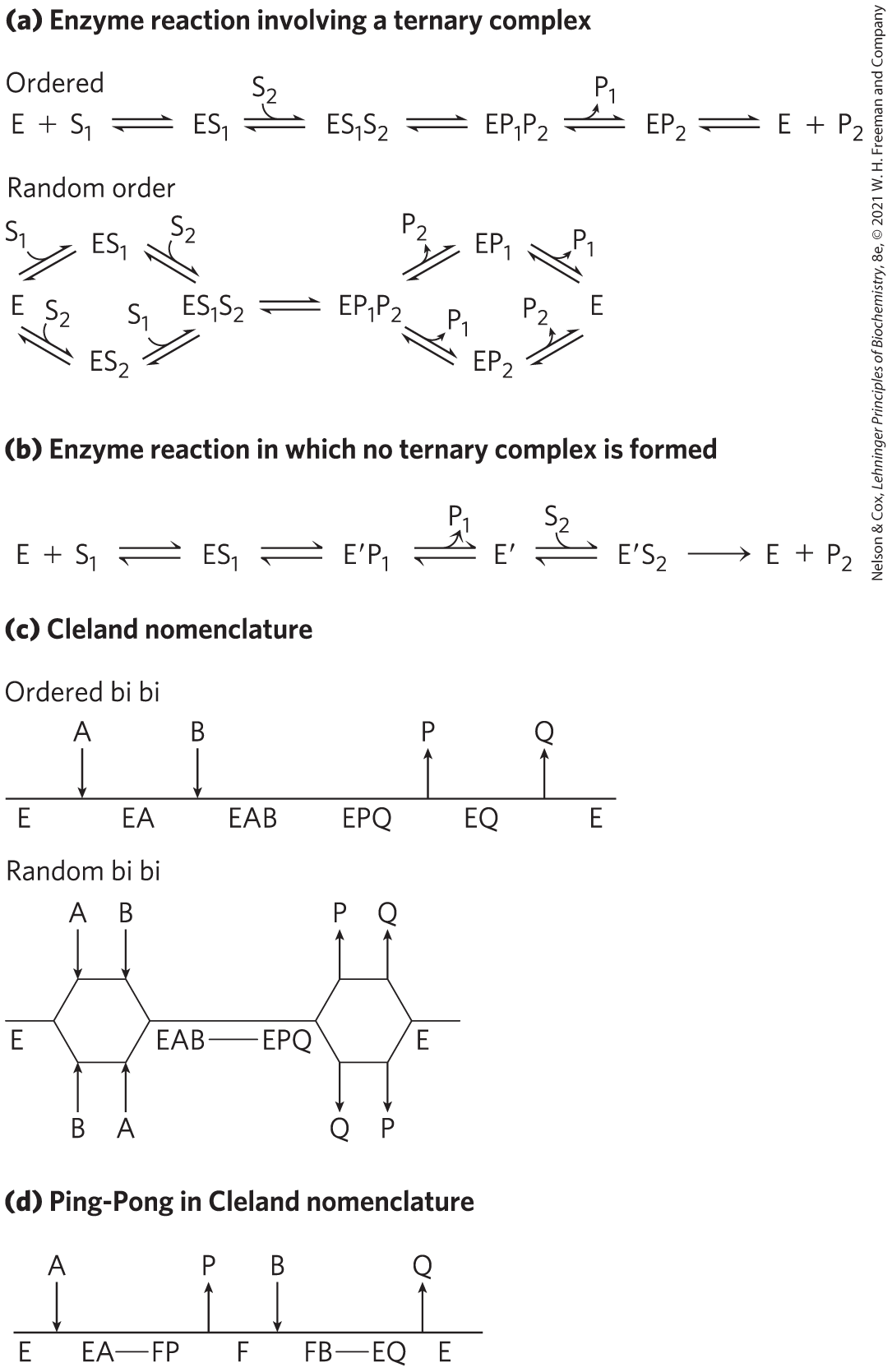
FIGURE 6-15 Common mechanisms for enzyme-catalyzed bisubstrate reactions. (a) The enzyme and both substrates come together to form a ternary complex. In ordered binding, substrate 1 must bind before substrate 2 can bind productively. In random binding, the substrates can bind in either order. Product dissociation can also be ordered or random. (b) An enzyme-substrate complex forms, a product leaves the complex, the altered enzyme forms a second complex with another substrate molecule, and the second product leaves, regenerating the enzyme. Substrate 1 may transfer a functional group to the enzyme (to form the covalently modified ), which is subsequently transferred to substrate 2. This is called a Ping-Pong or double-displacement mechanism. (c) Ternary complex formation depicted using Cleland nomenclature. In the ordered bi bi and random bi bi reactions shown here, the release of product follows the same pattern as the binding of substrate — both ordered or both random. (d) The Ping-Pong or double-displacement reaction described with Cleland nomenclature.
A shorthand notation developed by W. W. Cleland can be helpful in describing reactions with multiple substrates and products. In this system, referred to as Cleland nomenclature, substrates are denoted A, B, C, and D, in the order in which they bind to the enzyme, and products are denoted P, Q, S, and T, in the order in which they dissociate. Enzymatic reactions with one, two, three, or four substrates are referred to as uni, bi, ter, and quad, respectively. The enzyme is, as usual, denoted E, but if it is modified in the course of the reaction, successive forms are denoted F, G, and so on. The progress of the reaction is indicated with a horizontal line, with successive chemical species indicated below it. If there is an alternative in the reaction path, the horizontal line is bifurcated. Steps involving binding and dissociating substrates and products are indicated with vertical lines.
Common reactions with two substrates and two products (bi bi) are described with the shorthand forms illustrated in Figure 6-15c for an ordered bi bi reaction and a random bi bi reaction. In the latter example, the release of product is also random, as indicated by the two sets of bifurcations. Rarely, the binding of substrates is ordered and the release of products is random, or vice versa, eliminating the bifurcation at one end or the other of the progress line. In a Ping-Pong reaction, lacking a ternary complex, the pathway has a transient second form of the enzyme, F (Fig. 6-15d). This is the form in which a group has been transferred from the first substrate, A, to create a transient covalent attachment to the enzyme. As noted above, such reactions are often called double-displacement reactions, as a group is transferred first from substrate A to the enzyme and then from the enzyme to substrate B. Substrates A and B do not encounter each other on the enzyme.
Michaelis-Menten steady-state kinetics can provide only limited information about the number of steps and intermediates in an enzymatic reaction, but the approach can be used to distinguish between pathways that have a ternary intermediate and pathways — including Ping-Pong pathways — that do not (Fig. 6-16). As we will see when we consider enzyme inhibition, steady-state kinetics can also distinguish between ordered and random binding of substrates and products in reactions with ternary intermediates.
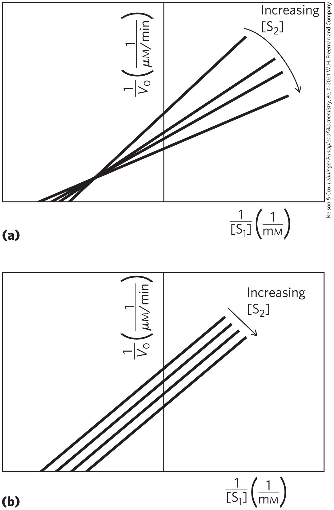
FIGURE 6-16 Steady-state kinetic analysis of bisubstrate reactions. In these double-reciprocal plots, the concentration of substrate 1 is varied while the concentration of substrate 2 is held constant. This is repeated for several values of , generating several separate lines. (a) Intersecting lines indicate that a ternary complex is formed in the reaction; (b) parallel lines indicate a Ping-Pong (double-displacement) pathway.
Enzyme Activity Depends on pH
In general, steady-state kinetics provides information required to characterize an enzyme and assess its catalytic efficiency. Additional information can be gained by examination of how the key experimental parameters and change when reaction conditions change, particularly pH. Enzymes have an optimum pH (or pH range) at which their activity is maximal (Fig. 6-17); at higher or lower pH, activity decreases. This is not surprising. Amino acid side chains in the active site may act as weak acids and bases only if they maintain a certain state of ionization. Elsewhere in the protein, removing a proton from a His residue, for example, might eliminate an ionic interaction that is essential for stabilizing the active conformation of the enzyme. A less common cause of pH sensitivity is titration of a group on the substrate.
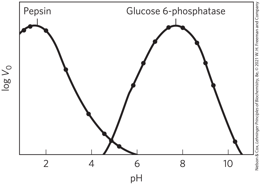
FIGURE 6-17 The pH-activity profiles of two enzymes. These curves are constructed from measurements of initial velocities when the reaction is carried out in buffers of different pH. Because pH is a logarithmic scale reflecting 10-fold changes in , the changes in are also plotted on a logarithmic scale. The pH optimum for the activity of an enzyme is generally close to the pH of the environment in which the enzyme is normally found. Pepsin, a peptidase found in the stomach, has a pH optimum of about 1.6. The pH of gastric juice is between 1 and 2. Glucose 6-phosphatase of hepatocytes (liver cells), with a pH optimum of about 7.8, is responsible for releasing glucose into the blood. The normal pH of the cytosol of hepatocytes is about 7.2.
The pH range over which an enzyme undergoes changes in activity can provide a clue to the type of amino acid residue involved (see Table 3-1). A change in activity near pH 7.0, for example, often reflects titration of a His residue. The effects of pH must be interpreted with some caution, however. In the closely packed environment of a protein, the of amino acid side chains can be significantly altered. For example, a nearby positive charge can lower the of a Lys residue, and a nearby negative charge can increase it. Such effects sometimes result in a that is shifted by several pH units from its value in the free amino acid. In the enzyme acetoacetate decarboxylase, for example, one Lys residue has a of 6.6 (compared with 10.5 in free lysine) due to electrostatic effects of nearby positive charges.
Pre–Steady State Kinetics Can Provide Evidence for Specific Reaction Steps
The mechanistic insight provided by steady-state kinetics can be augmented, sometimes dramatically, by an examination of the pre–steady state. Consider an enzyme with a reaction mechanism that conforms to the scheme in Equation 6-28, featuring three steps:
Overall catalytic efficiency for this reaction can be assessed with steady-state kinetics, but the rates of the individual steps cannot be determined in this way, and the slow (rate-limiting) step can rarely be identified. For the rate constants of individual steps to be measured, the reaction must be studied during its pre–steady state. The first turnover of an enzyme-catalyzed reaction often occurs in seconds or milliseconds, so researchers use special equipment that allows mixing and sampling on this time scale (Fig. 6-18a). Reactions are stopped and protein-bound products are quantified, after the timed addition and rapid mixing of an acid that denatures the protein and releases all bound molecules. A detailed description of pre–steady state kinetics is beyond the scope of this text, but we can illustrate the power of this approach by a simple example of an enzyme that uses the pathway shown in Equation 6-28. This example also involves an enzyme that catalyzes a relatively slow reaction, so the pre–steady state is more conveniently observed.
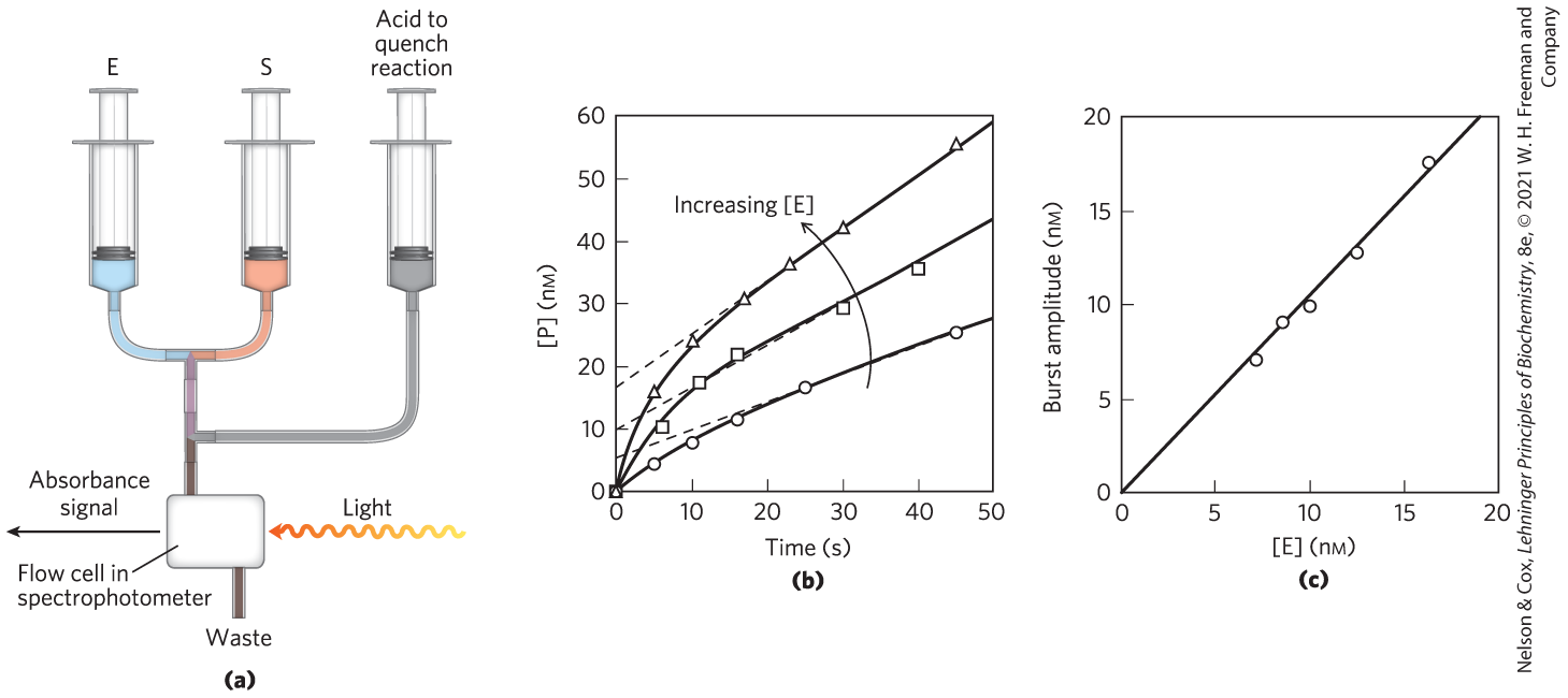
FIGURE 6-18 Pre–steady state kinetics. The transient phase that constitutes the pre–steady state often exists for mere seconds or milliseconds, requiring specialized equipment to monitor it. (a) A simple schematic for a rapid-mixing device, called a stopped-flow device. Enzyme (E) and substrate (S) are mixed with the aid of mechanically operated syringes. The reaction is quenched at a programmed time by adding a denaturing acid through another syringe, and the amount of product formed is measured, in this case with a spectrophotometer. (b) Experimental data for an enzyme reaction show the pre–steady state occurring in the first 5 to 10 seconds. This is a relatively slow reaction and is used as an example because the steady state can be conveniently monitored. The slope of the lines after 15 seconds reflects the steady state. Extrapolating this slope back to zero time (dashed lines) gives the amplitude of the burst phase. The progress of the reaction during the pre–steady state primarily reflects the chemical steps in the reaction (details of which are not shown). The presence of a burst implies that a step following the chemical step that produces P is rate-limiting — in this case, the product-release step. Notice that the extrapolated intercept at time = 0 increases as [E] increases. (c) A plot of burst amplitude (the intercepts from (b)) versus [E] shows that one molecule of P is formed in each active site during the burst (pre–steady state) phase. This provides evidence that product release is the rate-limiting step, because it is the only step following product formation in this simple enzymatic reaction. The enzyme used in this experiment was RNase P, one of the catalytic RNAs described in Chapter 26. [(b, c) Data from J. Hsieh et al., RNA 15:224, 2009.]
For many enzymes, dissociation of product is rate-limiting. In this example (Fig. 6-18b, c), the rate of dissociation of the product is slower than the rate of its formation . Product dissociation therefore dictates the rates observed in the steady state. How do we know that is rate-limiting? A slow gives rise to a burst of product formation in the pre–steady state, because the preceding steps are relatively fast. The burst reflects the rapid conversion of one molecule of substrate to one molecule of product at each enzyme active site. The observed rate of product formation soon slows to the steady-state rate as the bound product is slowly released. Each enzymatic turnover after the first one must proceed through the slow product-release step. However, the rapid generation of product in that first turnover provides much information. The amplitude of the burst — when one molecule of product is generated per molecule of enzyme present (Fig. 6-18c), measured by extrapolating the steady-state progress line back to zero time — is the highest amplitude possible. This provides one piece of evidence that product release is, indeed, rate-limiting. The rate constant for the chemical reaction step, , can be derived from the observed rate of the burst phase.
Of course, enzymes do not always conform to the simple reaction scheme of Equation 6-28. Formally, the observation of a burst indicates that a rate-limiting step (typically, product release, or an enzyme conformational change, or another chemical step) occurs after formation of the product being monitored. Additional experiments and analysis can often define the rates of each step in a multistep enzymatic reaction. Some examples of the application of pre–steady state kinetics are included in the descriptions of specific enzymes in Section 6.4.
Enzymes Are Subject to Reversible or Irreversible Inhibition
Enzyme inhibitors are molecules that interfere with catalysis, slowing or halting enzymatic reactions. Enzymes catalyze virtually all cellular processes, so it should not be surprising that enzyme inhibitors are among the most important pharmaceutical agents known. For example, aspirin (acetylsalicylate) inhibits the enzyme that catalyzes the first step in the synthesis of prostaglandins, compounds involved in many processes, including some that produce pain. The study of enzyme inhibitors also has provided valuable information about enzyme mechanisms and has helped define some metabolic pathways. There are two broad classes of enzyme inhibitors: reversible and irreversible.
Reversible Inhibition
One common type of reversible inhibition is called competitive (Fig. 6-19a). A competitive inhibitor competes with the substrate for the active site of an enzyme. While the inhibitor (I) occupies the active site, the substrate is excluded, and vice versa. Many competitive inhibitors are structurally similar to the substrate and combine with the enzyme to form an unreactive EI complex. Even fleeting combinations of this type will reduce the efficiency of an enzyme. Competitive inhibition can be analyzed quantitatively by steady-state kinetics. In the presence of a competitive inhibitor, the Michaelis-Menten equation (Eqn 6-9) becomes
(6-31)
where
Equation 6-31 describes the important features of competitive inhibition. The experimentally determined variable , the observed in the presence of the inhibitor, is often called the “apparent” .
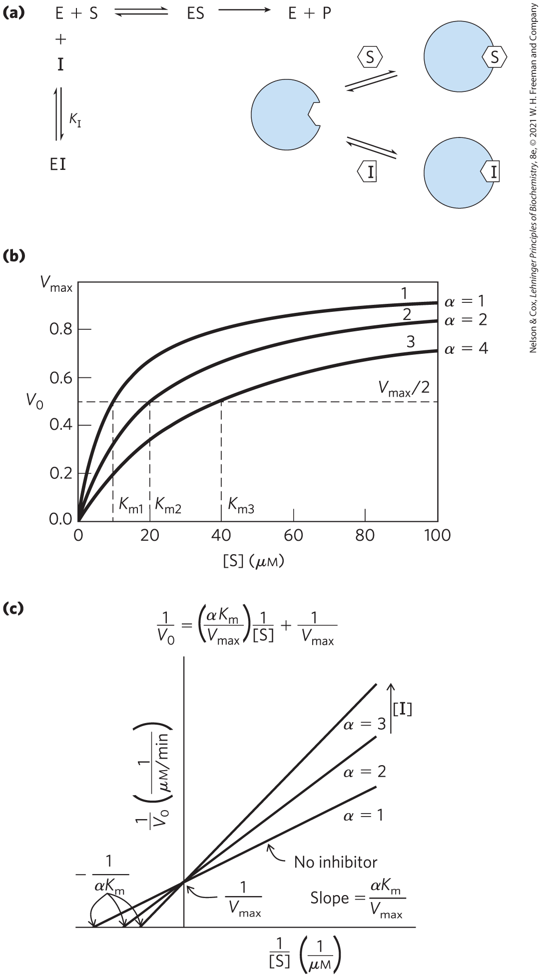
FIGURE 6-19 Competitive inhibition. (a) Competitive inhibitors bind to the enzyme’s active site; is the equilibrium dissociation constant for inhibitor binding to E. (b) Competitive inhibitors affect the observed , but not the . This is readily evident in the plot of versus [S]. (c) In a Lineweaver-Burk plot, the lines generated + and − inhibitor intersect on the y axis, which reflects . As the observed increases in the presence of an inhibitor, the intercept on the x axis moves to the right.
Bound inhibitor does not inactivate the enzyme. When the inhibitor dissociates, substrate can bind and react. Because the inhibitor binds reversibly to the enzyme, the competition can be biased to favor the substrate simply by adding more substrate. When [S] far exceeds [I], the probability that an inhibitor molecule will bind to the enzyme is minimized and the reaction exhibits normal . However, in the presence of inhibitor, the [S] at which , the apparent , increases in the presence of inhibitor by the factor α (Fig. 6-19b). This effect on apparent , combined with the absence of an effect on , is diagnostic of competitive inhibition and is readily revealed in a double-reciprocal plot (Fig. 6-19c). The equilibrium constant for inhibitor binding, , can be obtained from the same plot.
A medical therapy based on competition at the active site is used to treat patients who have ingested methanol, a solvent found in gas-line antifreeze. The liver enzyme alcohol dehydrogenase converts methanol to formaldehyde, which is damaging to many tissues. Blindness is a common result of methanol ingestion, because the eyes are particularly sensitive to formaldehyde. Ethanol competes effectively with methanol as an alternative substrate for alcohol dehydrogenase. The effect of ethanol is much like that of a competitive inhibitor, with the distinction that ethanol is also a substrate for alcohol dehydrogenase and its concentration will decrease over time as the enzyme converts it to acetaldehyde. The therapy for methanol poisoning is slow intravenous infusion of ethanol, at a rate that maintains a controlled concentration in the blood for several hours. This slows the formation of formaldehyde, lessening the danger while the kidneys filter out the methanol to be excreted harmlessly in the urine.
 A medical therapy based on competition at the active site is used to treat patients who have ingested methanol, a solvent found in gas-line antifreeze. The liver enzyme alcohol dehydrogenase converts methanol to formaldehyde, which is damaging to many tissues. Blindness is a common result of methanol ingestion, because the eyes are particularly sensitive to formaldehyde. Ethanol competes effectively with methanol as an alternative substrate for alcohol dehydrogenase. The effect of ethanol is much like that of a competitive inhibitor, with the distinction that ethanol is also a substrate for alcohol dehydrogenase and its concentration will decrease over time as the enzyme converts it to acetaldehyde. The therapy for methanol poisoning is slow intravenous infusion of ethanol, at a rate that maintains a controlled concentration in the blood for several hours. This slows the formation of formaldehyde, lessening the danger while the kidneys filter out the methanol to be excreted harmlessly in the urine.
Two other types of reversible inhibition, uncompetitive and mixed, can be defined in terms of one-substrate enzymes, but in practice are observed only with enzymes having two or more substrates. An uncompetitive inhibitor (Fig. 6-20a) binds at a site distinct from the substrate active site and, unlike a competitive inhibitor, binds only to the ES complex. In the presence of an uncompetitive inhibitor, the Michaelis-Menten equation is altered to
(6-32)
where
As described by Equation 6-32, at high concentrations of substrate, approaches . Thus, an uncompetitive inhibitor lowers the measured . Apparent also decreases, because the [S] required to reach one-half decreases by the factor (Fig. 6-20b, c). This behavior can be explained as follows. Because the enzyme is inactive when the uncompetitive inhibitor is bound, but the inhibitor is not competing with substrate for binding, the inhibitor effectively removes some fraction of the enzyme molecules from the reaction. Given that depends on [E], the observed decreases. Given that the inhibitor binds only to the ES complex, only ES (not free enzyme) is deleted from the reaction, so the [S] needed to reach — that is, — declines by the same amount.
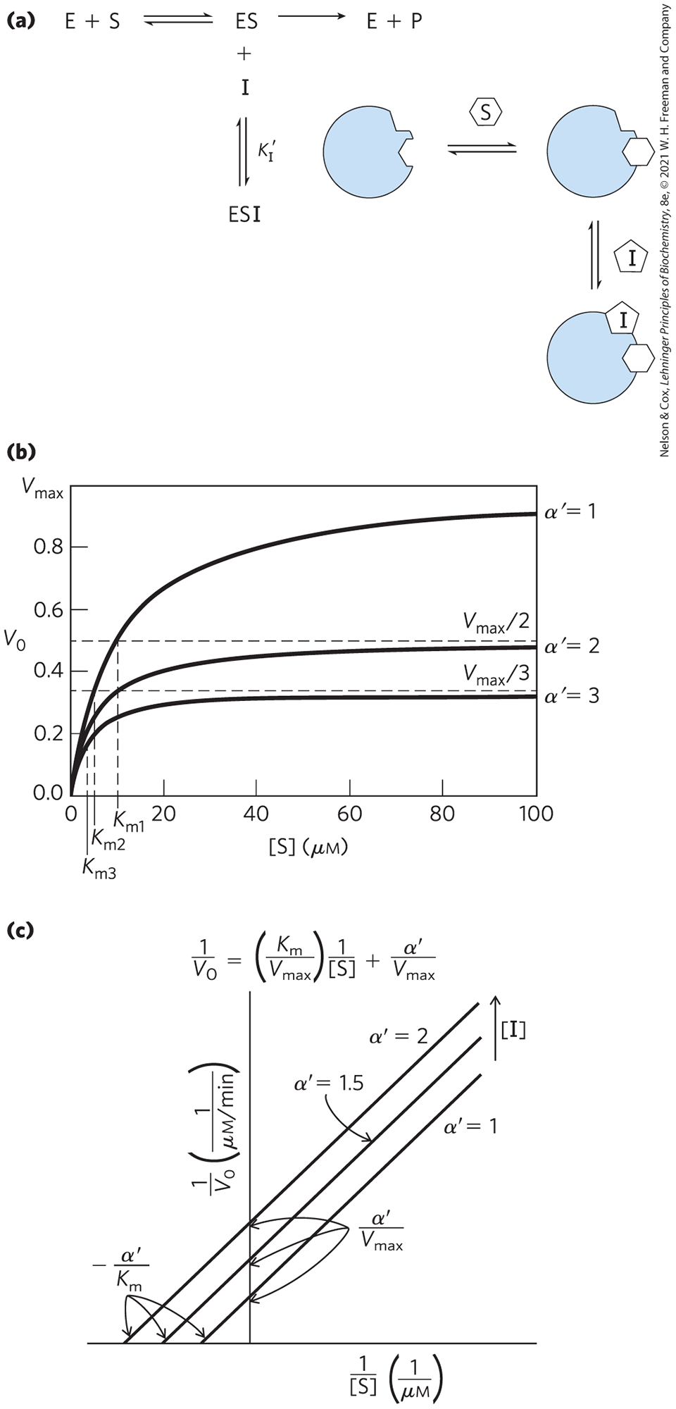
FIGURE 6-20 Uncompetitive inhibition. (a) Uncompetitive inhibitors bind at a separate site, but bind only to the ES complex; is the equilibrium constant for an inhibitor binding to ES. (b) In the presence of an uncompetitive inhibitor, both the and the decline, and by equivalent factors. In the versus [S] plot, the decline in is somewhat easier to discern than the decline in . (c) The Lineweaver-Burk plot for an uncompetitive inhibitor is quite diagnostic, as the lines generated in the presence and absence of an inhibitor are parallel. Note that the lines seen in the presence of an inhibitor are always above the line generated in the absence of an inhibitor, reflecting the decline in both and brought about by the inhibitor (i.e., the intercepts move up on the y axis and to the left on the x axis).
A mixed inhibitor (Fig. 6-21a) also binds at a site distinct from the substrate active site, but it binds to either E or ES. The rate equation describing mixed inhibition is
(6-33)
where α and are defined as above. A mixed inhibitor usually affects both and (Fig. 6-21b, c). is affected because the inhibitor renders some fraction of the available enzyme molecules inactive, lowering the effective [E] on which depends. The may increase or decrease, depending on which enzyme form, E or ES, the inhibitor binds to most strongly. The special case of , rarely encountered in experiments, historically has been defined as noncompetitive inhibition. Examine Equation 6-33 to see why a noncompetitive inhibitor would affect the but not the .
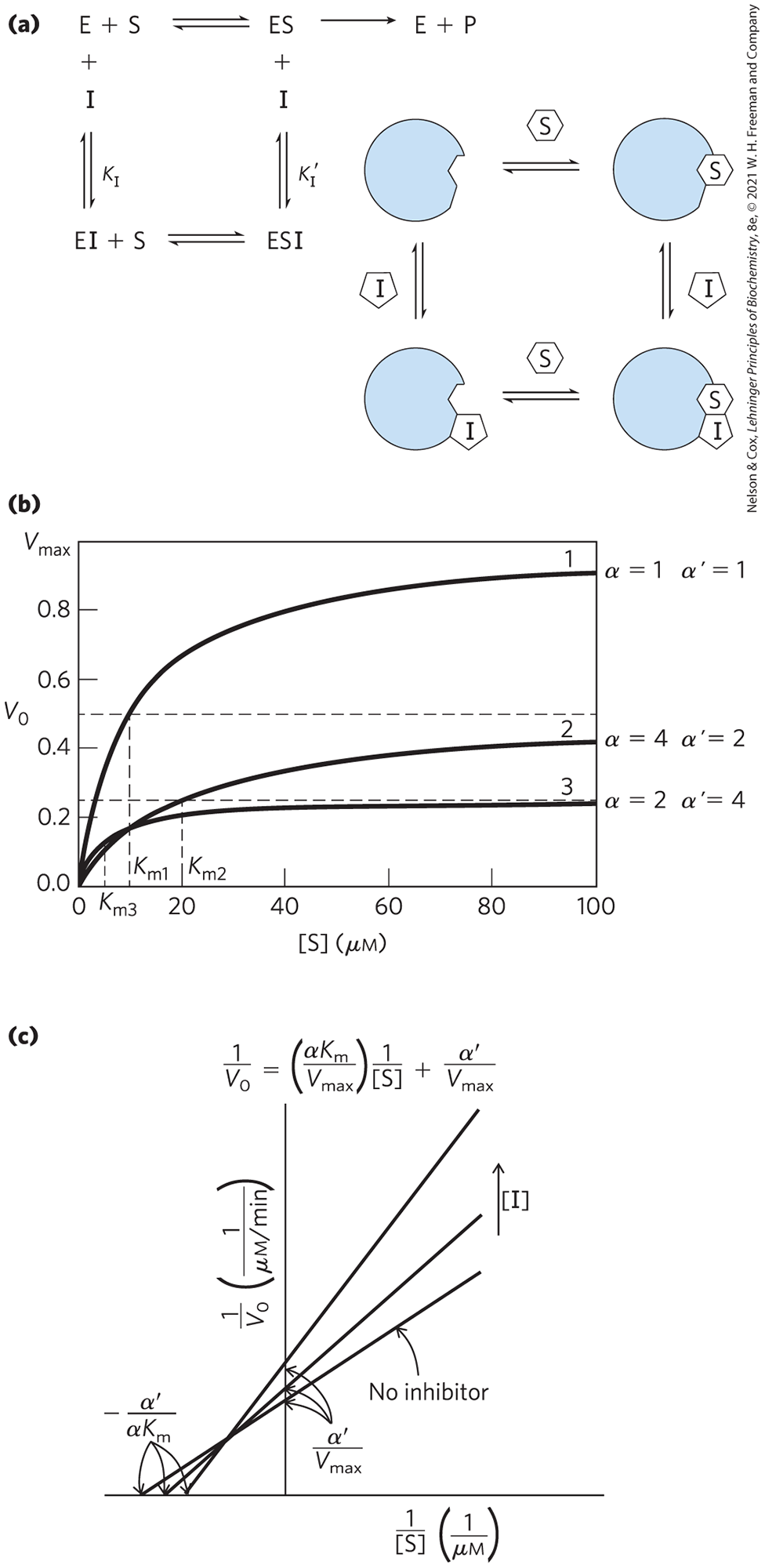
FIGURE 6-21 Mixed inhibition. (a) Mixed inhibitors bind at a separate site, but they may bind to either E or ES. (b) The kinetic patterns brought about by a mixed inhibitor are complex. The always declines. The may increase or decrease, depending upon the relative values of α and . (c) In a Lineweaver-Burk plot, the lines generated + and − inhibitor always intersect, but not on an axis. The intercepts on the y axis always move up, as the declines. The lines may intersect either above or below the x axis. When they intersect above, as shown here, and the observed is increasing. When the lines intersect below the x axis (not shown), and the observed is decreasing.
Equation 6-33 is a general expression for the effects of reversible inhibitors, simplifying to the expressions for competitive inhibition and uncompetitive inhibition when or α = 1.0, respectively. From this expression we can summarize the effects of inhibitors on individual kinetic parameters. For all reversible inhibitors, the apparent , because the right side of Equation 6-33 always simplifies to at sufficiently high substrate concentrations. For competitive inhibitors, and can thus be ignored. Taking this expression for apparent , we can also derive a general expression for apparent to show how this parameter changes in the presence of reversible inhibitors. Apparent , as always, equals the [S] at which is one-half apparent or, more generally, when . This condition is met when . Thus, apparent . The terms α and reflect the binding of inhibitor to E and ES, respectively. Thus, the term is a mathematical expression of the relative affinity of inhibitor for the two enzyme forms. This expression is simpler when either α or is 1.0 (for uncompetitive or competitive inhibitors), as summarized in Table 6-9.
| Inhibitor type | Apparent | Apparent |
|---|---|---|
| None | ||
| Competitive | ||
| Uncompetitive | ||
| Mixed |
In practice, uncompetitive inhibition and mixed inhibition are observed only for enzymes with two or more substrates — say, and — and are very important in the experimental analysis of such enzymes. If an inhibitor binds to the site normally occupied by , it may act as a competitive inhibitor in experiments in which is varied. If an inhibitor binds to the site normally occupied by , it may act as a mixed or uncompetitive inhibitor of . The actual inhibition patterns observed depend on whether the - and -binding events are ordered or random, and thus the order in which substrates bind and products leave the active site can be determined. Product inhibition experiments in which one of the reaction products is provided as an inhibitor are often particularly informative. If only one of two reaction products is present, no reverse reaction can take place. However, a product generally binds to some part of the active site and can thus serve as an effective inhibitor. Enzymologists can combine steady-state kinetic studies involving different combinations and amounts of products and inhibitors with pre–steady state analysis to develop a detailed picture of the mechanism of a bisubstrate reaction.
WORKED EXAMPLE 6-3 Effect of Inhibitor on
The researchers working on happyase (see Worked Examples 6-1 and 6-2) discover that the compound STRESS is a potent competitive inhibitor of happyase. Addition of 1 nm STRESS increases the measured for SAD by a factor of 2. What are the values for α and under these conditions?
SOLUTION:
Recall that the apparent , the measured in the presence of a competitive inhibitor, is defined as . Because for SAD increases by a factor of 2 in the presence of 1 nmSTRESS, the value of α must be 2. The value of for a competitive inhibitor is 1, by definition.
Irreversible Inhibition
The irreversible inhibitors bind covalently with or destroy a functional group on an enzyme that is essential for the enzyme’s activity, or they form a highly stable noncovalent association. Formation of a covalent link between an irreversible inhibitor and an enzyme is a particularly effective way to inactivate an enzyme. Irreversible inhibitors are another useful tool for studying reaction mechanisms. Amino acids with key catalytic functions in the active site can sometimes be identified by determining which residue is covalently linked to an inhibitor after the enzyme is inactivated. An example is shown in Figure 6-22.
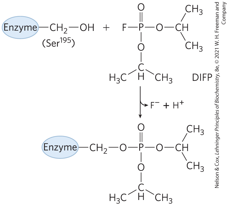
FIGURE 6-22 Irreversible inhibition. Reaction of chymotrypsin with diisopropylfluorophosphate (DIFP) modifies and irreversibly inhibits the enzyme. This has led to the conclusion that is the key active-site Ser residue in chymotrypsin.
A special class of irreversible inhibitors is the suicide inactivators. These compounds are relatively unreactive until they bind to the active site of a specific enzyme. A suicide inactivator undergoes the first few chemical steps of the normal enzymatic reaction, but instead of being transformed into the normal product, the inactivator is converted to a very reactive compound that combines irreversibly with the enzyme. These compounds are also called mechanism-based inactivators, because they hijack the normal enzyme reaction mechanism to inactivate the enzyme. Suicide inactivators play a significant role in rational drug design, an approach to obtaining new pharmaceutical agents in which chemists synthesize novel substrates based on knowledge of substrates and reaction mechanisms. A well-designed suicide inactivator is specific for a single enzyme and is unreactive until it is within that enzyme’s active site, so drugs based on this approach can offer the important advantage of few side effects (Box 6-1).
An irreversible inhibitor need not bind covalently to the enzyme. Noncovalent binding is enough, if that binding is so tight that the inhibitor dissociates only rarely. How does a chemist develop a tight-binding inhibitor? Recall that enzymes evolve to bind most tightly to the transition states of the reactions that they catalyze. In principle, if one can design a molecule that looks like that reaction transition state, it should bind tightly to the enzyme. Even though transition states cannot be observed directly, chemists can often predict the approximate structure of a transition state based on accumulated knowledge about reaction mechanisms. Although the transition state is by definition transient and thus unstable, in some cases stable molecules can be designed that resemble transition states. These are called transition-state analogs. They bind to an enzyme more tightly than does the substrate in the ES complex, because they fit into the active site better (that is, they form a greater number of weak interactions) than the substrate itself.
 Recall that enzymes evolve to bind most tightly to the transition states of the reactions that they catalyze. In principle, if one can design a molecule that looks like that reaction transition state, it should bind tightly to the enzyme. Even though transition states cannot be observed directly, chemists can often predict the approximate structure of a transition state based on accumulated knowledge about reaction mechanisms. Although the transition state is by definition transient and thus unstable, in some cases stable molecules can be designed that resemble transition states. These are called
 The idea of transition-state analogs was suggested by Linus Pauling in the 1940s, and it has been explored using a variety of enzymes. For example, transition-state analogs designed to inhibit the glycolytic enzyme aldolase bind to that enzyme more than four orders of magnitude more tightly than do its substrates (Fig. 6-23). A transition-state analog cannot perfectly mimic a transition state. Some analogs, however, bind to a target enzyme to times more tightly than does the normal substrate, providing good evidence that enzyme active sites are indeed complementary to transition states. The concept of transition-state analogs is important to the design of new pharmaceutical agents. As we shall see in Section 6.4, the powerful anti-HIV drugs called protease inhibitors were designed in part as tight-binding transition-state analogs.
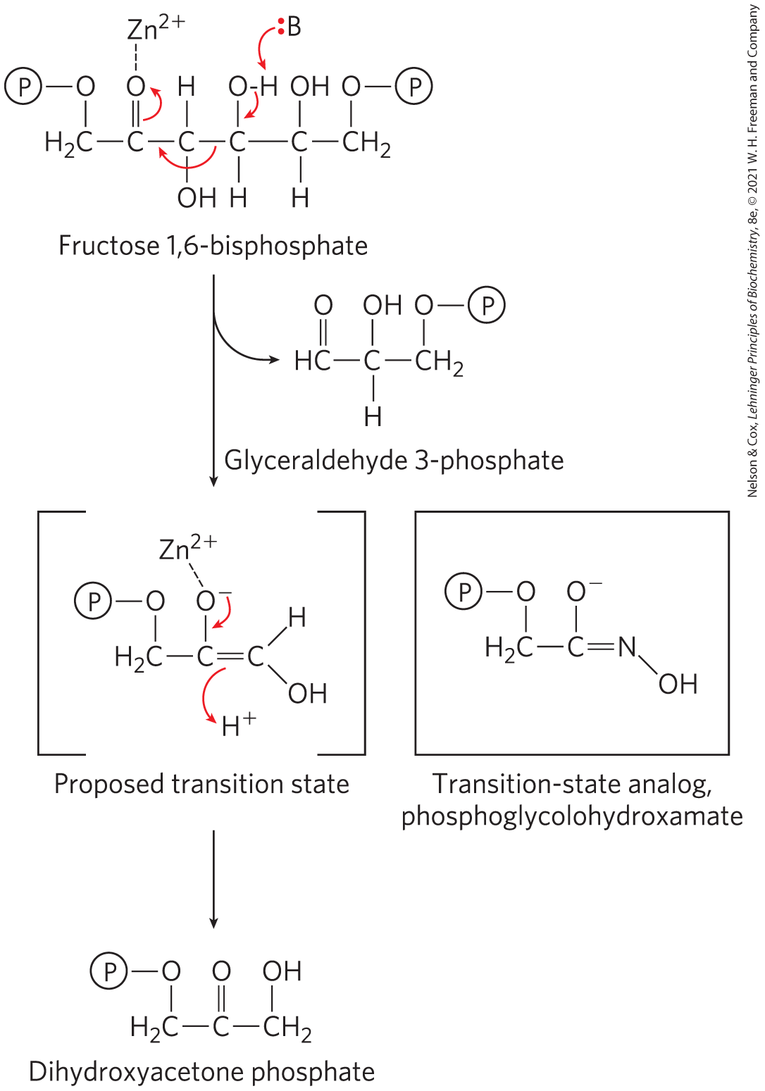
FIGURE 6-23 A transition-state analog. In glycolysis, a class II aldolase (found in bacteria and fungi) catalyzes the cleavage of fructose 1,6-bisphosphate to form glyceraldehyde 3-phosphate and dihydroxyacetone phosphate. The reaction proceeds via a reverse aldol-like mechanism. The compound phosphoglycolohydroxamate, which resembles the proposed enediolate transition state, binds to the enzyme nearly 10,000 times better than does the dihydroxyacetone phosphate product.
SUMMARY 6.3 Enzyme Kinetics as an Approach to Understanding Mechanism
- Most enzymes have certain kinetic properties in common. When substrate is added to an enzyme, the reaction rapidly achieves a steady state in which the rate at which the ES complex forms balances the rate at which it breaks down. As [S] increases, the steady-state activity of a fixed concentration of enzyme increases in a hyperbolic fashion to approach a characteristic maximum rate, , at which essentially all the enzyme has formed a complex with substrate.
- The Michaelis-Menten equation
relates initial velocity to [S] and through the Michaelis constant, . Michaelis-Menten kinetics is also called steady-state kinetics. and have different meanings for different enzymes. However, the is always equal to the substrate concentration that results in a reaction rate equal to one-half .
- The values of and can be determined by using transformations of the Michaelis-Menten equation that allow linear plotting of data and extrapolation (for example, Lineweaver-Burk), or (more accurately) by using nonlinear regression.
- The limiting rate of an enzyme-catalyzed reaction at saturation is described by the constant , the turnover number. The ratio provides a good measure of catalytic efficiency.
- Most enzymes catalyze reactions involving multiple substrates, with the majority having two substrates and two products. The Michaelis-Menten equation is applicable to bisubstrate reactions, which occur by ternary complex or Ping-Pong (double-displacement) pathways.
- Every enzyme has an optimum pH (or pH range) at which it has maximal activity. The pH-rate profile can provide mechanistic clues.
- Pre–steady state kinetics can provide added insight into enzymatic reaction mechanisms.
- Reversible inhibition of an enzyme may be competitive, uncompetitive, or mixed. Competitive inhibitors compete with substrate by binding reversibly to the active site, but they are not transformed by the enzyme. Uncompetitive inhibitors bind only to the ES complex, at a site distinct from the active site. Mixed inhibitors bind to either E or ES, again at a site distinct from the active site. In irreversible inhibition, an inhibitor binds permanently to an active site by forming a covalent bond or a very stable noncovalent interaction. Inhibition patterns can elucidate mechanism.
 Most enzymes have certain kinetic properties in common. When substrate is added to an enzyme, the reaction rapidly achieves a steady state in which the rate at which the ES complex forms balances the rate at which it breaks down. As [S] increases, the steady-state activity of a fixed concentration of enzyme increases in a hyperbolic fashion to approach a characteristic maximum rate, , at which essentially all the enzyme has formed a complex with substrate.