4.5 Determination of Protein and Biomolecular Structures
In this chapter we have presented many types of protein structures. How were these structures determined? Structural biology is the study of the three-dimensional structures of biomolecules, including proteins, nucleic acids, lipid membranes, and oligosaccharides. Structural biologists combine biochemical approaches with physical tools and computational methods to obtain these structures. Structural biology is extraordinarily powerful for elucidating the relationships between the structure and function of proteins, the molecular basis for enzymatic catalysis and ligand binding, and evolutionary relationships between proteins. Here we focus primarily on three commonly used methods in structural biology: x-ray crystallography, nuclear magnetic resonance (NMR), and cryo-electron microscopy (cryo-EM). Which method a structural biologist uses depends on the system being studied and what information is to be learned. Often structural biologists combine multiple methods to provide a more complete view of function.
 Structural biology is the study of the three-dimensional structures of biomolecules, including proteins, nucleic acids, lipid membranes, and oligosaccharides. Structural biologists combine biochemical approaches with physical tools and computational methods to obtain these structures. Structural biology is extraordinarily powerful for elucidating the relationships between the structure and function of proteins, the molecular basis for enzymatic catalysis and ligand binding, and evolutionary relationships between proteins. Here we focus primarily on three commonly used methods in structural biology: x-ray crystallography, nuclear magnetic resonance (NMR), and cryo-electron microscopy (cryo-EM). Which method a structural biologist uses depends on the system being studied and what information is to be learned. Often structural biologists combine multiple methods to provide a more complete view of function.
Increasingly, computational methods such as molecular dynamics simulations and in silico protein folding are proving to be essential for structural biologists, and these are discussed in Box 4-5.
X-ray Diffraction Produces Electron Density Maps from Protein Crystals
The spacing of atoms in a crystal lattice can be determined by measuring the locations and intensities of spots produced on a detector by a beam of x-rays of given wavelength, after the beam has been diffracted by the electrons of the atoms. For example, x-ray analysis of sodium chloride crystals shows that and ions are arranged in a simple cubic lattice. The spacing of the different kinds of atoms in complex organic molecules, even very large ones such as proteins, can also be analyzed by x-ray diffraction methods. However, the technique for analyzing crystals of complex molecules is far more laborious than the technique for analyzing simple salt crystals. When the repeating pattern of the crystal is a molecule as large as, say, a protein, the numerous atoms in the molecule yield thousands of diffraction spots that must be analyzed by computer.
Consider how images are generated in a light microscope. Light from a point source is focused on an object. The object scatters the light waves, and these scattered waves are recombined by a series of lenses to generate an enlarged image of the object. The smallest object whose structure can be determined by such a system — that is, the resolving power of the microscope — is determined by the wavelength of the light, in this case visible light, with wavelengths in the range of 400 to 700 nm. Objects smaller than half the wavelength of the incident light cannot be resolved. To resolve objects as small as proteins we must use x-rays, with wavelengths in the range of 0.7 to 1.5 Å (0.07 to 0.15 nm). However, there are no lenses that can recombine x-rays to form an image; instead, the pattern of diffracted x-rays is collected directly and an image is reconstructed by mathematical techniques.
The amount of information obtained from x-ray crystallography depends on the degree of structural order in the sample. Some important structural parameters were obtained from early studies of the diffraction patterns of the fibrous proteins arranged in regular arrays in hair and wool. However, the orderly bundles formed by fibrous proteins are not crystals — the molecules are aligned side by side, but not all are oriented in the same direction. More-detailed three-dimensional structural information about proteins requires a highly ordered protein crystal. The structures of many proteins are not yet known, simply because they have proved difficult to crystallize. Practitioners have compared making protein crystals to holding together a stack of bowling balls with cellophane tape.
Operationally, there are several steps in x-ray structural analysis (Fig. 4-30). A crystal is placed in an x-ray beam between the x-ray source and a detector, and a regular array of spots, called reflections, is generated. The spots are created by the diffracted x-ray beam, and each atom in a molecule makes a contribution to each spot. An electron-density map of the protein is reconstructed from the overall diffraction pattern of spots by a mathematical technique called a Fourier transform. In effect, the computer acts as a “computational lens.” A model for the structure is then built that is consistent with the electron-density map.
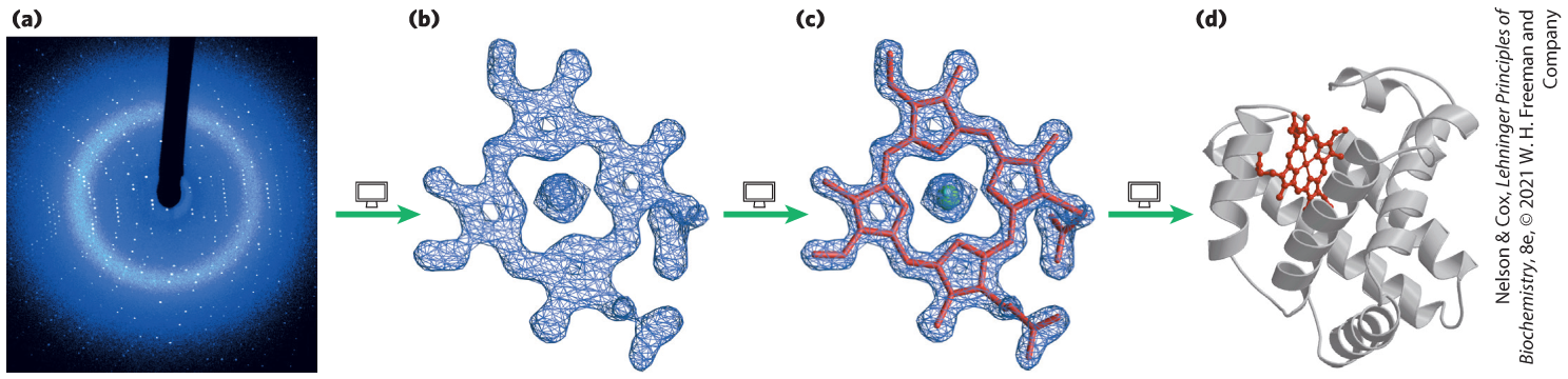
FIGURE 4-30 Steps in determining the structure of sperm whale myoglobin by x-ray crystallography. (a) X-ray diffraction patterns are generated from a crystal of the protein. (b) Data extracted from the diffraction patterns are used to calculate a three-dimensional electron-density map. The electron density of only part of the structure, the heme, is shown here. (c) Regions of greatest electron density reveal the location of atomic nuclei, and this information is used to piece together the final structure. Here, the heme structure is modeled into its electron-density map. (d) The completed structure of sperm whale myoglobin, including the heme. [(a, b, c) Photo and data from George N. Phillips, Jr., University of Wisconsin–Madison, Department of Biochemistry. (d) Data from PDB ID 2MBW, E. A. Brucker et al., J. Biol. Chem. 271:25,419, 1996.]
John Kendrew found that the x-ray diffraction pattern of crystalline myoglobin (isolated from muscles of the sperm whale) is highly complex, with nearly 25,000 reflections. Computer analysis of these reflections took place in stages. The resolution improved at each stage until, in 1959, the positions of virtually all the nonhydrogen atoms in the protein had been determined. The amino acid sequence of the protein, obtained by chemical analysis, was consistent with the molecular model. Over 100,000 protein structures, many of them much more complex than myoglobin, have since been determined to a similar level of resolution by x-ray crystallography.
The physical environment in a crystal, of course, is not identical to that in solution or in a living cell. A crystal imposes a space and time average on the structure deduced from its analysis, and x-ray diffraction studies provide little information about molecular motion within the protein. The conformation of proteins in a crystal can also be affected by nonphysiological factors such as incidental protein-protein contacts within the crystal. However, when structures derived from the analysis of crystals are compared with structural information obtained by other means (such as NMR, as described below), the crystal-derived structure almost always represents a functional conformation of the protein.
Distances between Protein Atoms Can Be Measured by Nuclear Magnetic Resonance
An advantage of nuclear magnetic resonance (NMR) studies is that they are carried out on macromolecules in solution, whereas x-ray crystallography is limited to molecules that can be crystallized. NMR can also illuminate the dynamic side of protein structure, including conformational changes, protein folding, and interactions with other molecules.
NMR is a manifestation of nuclear spin angular momentum, a quantum mechanical property of atomic nuclei. Only certain atoms, including , , , , and , have the kind of nuclear spin that gives rise to an NMR signal. Nuclear spin generates a magnetic dipole. When a strong, static magnetic field is applied to a solution containing a single type of macromolecule, the magnetic dipoles are aligned in the field in one of two orientations: parallel (low energy) or antiparallel (high energy). A short (∼10 μs) pulse of electromagnetic energy of suitable frequency (the resonant frequency, which is in the radio frequency range) is applied at right angles to the nuclei aligned in the magnetic field. Some energy is absorbed as nuclei switch to the high-energy state, and the absorption spectrum that results contains information about the identity of the nuclei and their immediate chemical environment. The data from many such experiments on a sample are averaged, increasing the signal-to-noise ratio, and an NMR spectrum such as that in Figure 4-31 is generated.
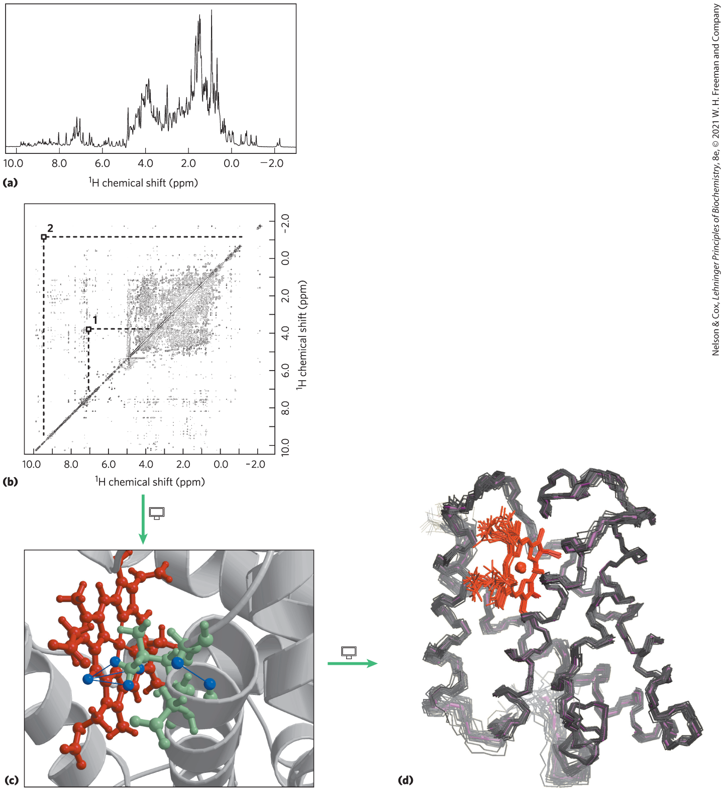
FIGURE 4-31 NMR spectra of a globin from a marine blood worm. (a) One-dimensional NMR spectrum. (b) Two-dimensional NMR data used to generate a three-dimensional structure of globin. The diagonal in a two-dimensional NMR spectrum is equivalent to a one-dimensional spectrum. The off-diagonal peaks are NOE signals generated by close-range interactions of atoms that may generate signals quite distant in the one-dimensional spectrum. Two such interactions are identified in (b), and their identities are shown with blue lines in (c). Three lines are drawn for interaction 2 between a methyl group in the protein and a hydrogen on the heme. The methyl group rotates rapidly such that each of its three hydrogens contributes equally to the interaction and the NMR signal. Such information is used to determine the complete three-dimensional structure, as in (d). The multiple lines shown for the protein backbone in (d) represent the family of structures consistent with the distance constraints in the NMR data. [Data from (a, b) B. F. Volkman, National Magnetic Resonance Facility at Madison; (c) PDB ID 1VRF; (d) PDB ID 1VRE, B. F. Volkman et al., Biochemistry 37:10,906, 1998.]
is particularly important in NMR experiments because of its high sensitivity and natural abundance. For macromolecules, NMR spectra can become quite complicated. Even a small protein has hundreds of atoms, typically resulting in a one-dimensional NMR spectrum too complex for analysis. Structural analysis of proteins became possible with the advent of two-dimensional NMR techniques (Fig. 4-31b, c, d). These methods allow measurement of distance-dependent coupling of nuclear spins in nearby atoms through space (the nuclear Overhauser effect (NOE), in a method dubbed NOESY) or the coupling of nuclear spins in atoms connected by covalent bonds (total correlation spectroscopy, or TOCSY).
Translating a two-dimensional NMR spectrum into a complete three-dimensional structure can be a laborious process. The NOE signals provide some information about the distances between individual atoms, but for these distance constraints to be useful, the atoms giving rise to each signal must be identified. Complementary TOCSY experiments can help identify which NOE signals reflect atoms that are linked by covalent bonds. Certain patterns of NOE signals have been associated with secondary structures such as α helices. Genetic engineering (Chapter 9) can be used to prepare proteins that contain the rare isotopes or . The new NMR signals produced by these atoms, and the coupling with signals resulting from these substitutions, help in the assignment of individual NOE signals. The process is also aided by a knowledge of the amino acid sequence of the polypeptide.
To generate a three-dimensional structure, researchers feed the distance constraints into a computer along with known geometric constraints such as chirality, van der Waals radii, and bond lengths and angles. The computer generates a family of closely related structures that represent the range of conformations consistent with the NOE distance constraints (Fig. 4-31d). The uncertainty in structures generated by NMR is in part a reflection of the molecular vibrations (known as breathing) within a protein structure in solution, discussed in more detail in Chapter 5. Normal experimental uncertainty can also play a role.
Thousands of Individual Molecules Are Used to Determine Structures by Cryo-Electron Microscopy
Our understanding of highly complex processes such as gene expression, mitochondrial respiration, or viral infection is aided immensely by knowing the detailed molecular structures of the proteins that participate in these processes. However, it is often difficult to determine the molecular structure of large, dynamic, macromolecular complexes that contain dozens of individual protein subunits. Moreover, integral membrane proteins often resist crystallization once they are removed from their lipid environment, making their structures difficult to solve by x-ray diffraction, and many are too large for NMR. In principle, discrete objects in the diameter range 100 to 300 Å can be visualized by electron microscopy (EM). In practice, the high intensity of the EM beam often damages the specimen before a high-resolution image can be obtained. In cryo-electron microscopy (cryo-EM), a sample containing many individual copies of the structure of interest is quick-frozen in vitreous (or noncrystalline) ice and kept frozen while being observed in two dimensions with the electron microscope, greatly reducing damage to the specimen by the electron beam.
Particles such as purified, multisubunit enzymes, arranged randomly on the microscope grid, are visualized with the cryo-electron microscope. When cryo-EM is combined with powerful algorithms for transforming the two-dimensional structures of tens of thousands of individual, randomly oriented complexes into a three-dimensional composite, it is sometimes possible to determine molecular structures at a level comparable to that obtained by x-ray crystallography (Fig. 4-32). In favorable cases, the repetitive aspects—choice of objects to be included in the analysis, imaging of each object individually, and calculations to produce a three-dimensional structure from the huge number of two-dimensional images—can be automated. The EMDataResource (www.emdataresource.org) is a unified resource for accessing structure maps deposited into data banks and assigned EMDataBank (EMDB) accession codes.
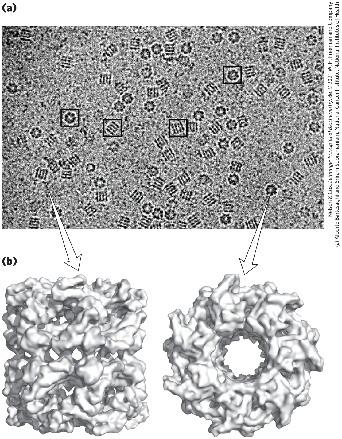
FIGURE 4-32 Structure of the chaperone protein GroEL as determined by single-particle cryo-EM. (a) Cryo-EM images of many individual GroEL particles. (b) Side and top views of the three-dimensional structure derived from analysis of the EM images. [(b) Data from PDB ID 3E76, P. D. Kaiser et al., Acta Crystallogr. 65:967, 2009.]
Many novel structures have now been obtained by cryo-EM without models based on prior x-ray or NMR structures. Since cryo-EM relies on imaging of single molecules of a complex, this technique can also be used to computationally sort the imaged particles and simultaneously determine structures of multiple conformational states. Cryo-EM has now been used to solve the structures of some of the most dynamic and largest molecular complexes in the cell, such as the human telomerase enzyme (Fig. 4-33). Telomerase is an essential enzyme for maintaining chromosome integrity in humans (see Chapter 26) and is the target of significant medical research due to its roles in aging and cancer. Cryo-EM was critical for the laboratories of Eva Nogales and Kathleen Collins in determining the architecture of telomerase due to the heterogeneity of the complex and because only minute quantities could be purified from human cells — far too little for crystallization, but enough to observe single molecules by cryo-EM.
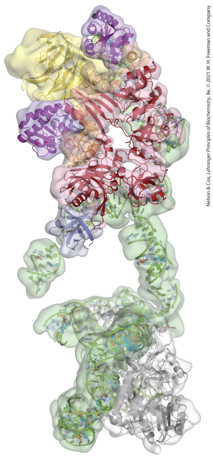
FIGURE 4-33 Cryo-EM structure of human telomerase. The structures of the RNA (green) and protein (ribbon representations) components of human telomerase are shown embedded in the calculated 10.2 Å EM density map. [Data from EMDB ID EMD-7521, T. Nguyen et al., Nature 557:190, 2018.]

Eva Nogales

Kathleen Collins
SUMMARY 4.5 Determination of Protein and Biomolecular Structures
- In x-ray crystallography, protein molecules are crystallized in well-ordered orientations that diffract x-rays. The patterns and intensities of the diffracted x-rays depend on the structure of the protein and its crystalline properties. Mathematical methods can then reconstruct the protein structure that produces a particular diffraction pattern.
- NMR is often carried out on molecules in solution and yields information about atomic nuclei and their chemical environment. Protein structures can be computed from NMR data using hundreds of distance and geometric constraints obtained from multi-dimensional NMR experiments.
- Biomolecules are frozen in vitreous ice for imaging by cryo-EM. The individual molecules are then identified and computationally sorted. The sorted two-dimensional images are then combined using computers to produce a three-dimensional structure.
 In x-ray crystallography, protein molecules are crystallized in well-ordered orientations that diffract x-rays. The patterns and intensities of the diffracted x-rays depend on the structure of the protein and its crystalline properties. Mathematical methods can then reconstruct the protein structure that produces a particular diffraction pattern.